

Loss is basically a penalty for a bad prediction. That is, loss is a number indicating how bad the model's prediction was on a single example. If the model's prediction is perfect, the loss is zero; otherwise, the loss is greater. The goal of training a model is to find a set of weights and biases that have low loss, on average, across all examples.
Loss functions are basically comparison between the predictions and the actual values using an error metric. This error indicates how the weights should be adjusted. The cost function is the average loss across the entire sample of data and predictions.
Algorithms is machine learning are either minimizing or maximizing a function, also called an "objective function". Loss functions are those which are minimized. A loss function is a measure on how good a model is in predicting the outcome with the most common method used to obtain the minimum is called "gradient descent".
Some of the factors affecting the choice of loss function are:
Loss functions can be categorized into two:
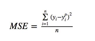
Also called the Mean Square Error Loss or Quadratic Loss. This is the most commonly used loss function for regression problems. MSE is the sum of squared distances between our target variable and predicted values.
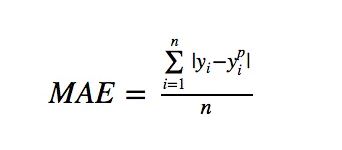
This is the sum of absolute differences between our target and predicted variables. So it measures the average magnitude of errors in a set of predictions, without considering their directions. (If we consider directions also, that would be called Mean Bias Error (MBE), which is a sum of residuals/errors). The range is also 0 to ∞.
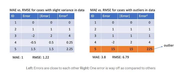
MAE Vs MSE (L1 Vs L2)
If we compare values for MAE and RMSE, since MSE squares the error (y — y_predicted = e), the value of error (e) increases a lot if e > 1. If we have an outlier in our data, the value of e will be high and e² will be >> |e|. This will make the model with MSE loss give more weight to outliers than a model with MAE loss. In the 2nd case above, the model with RMSE as loss will be adjusted to minimize that single outlier case at the expense of other common examples, which will reduce its overall performance.
Problem using MAE (L1)
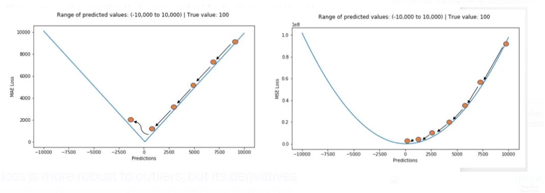
This is especially for neural networks, its gradient is the same throughout, which means the gradient will be large even for small loss values. This isn’t good for learning. To fix this, we can use dynamic learning rate which decreases as we move closer to the minima. MSE behaves nicely in this case and will converge even with a fixed learning rate. The gradient of MSE loss is high for larger loss values and decreases as loss approaches 0, making it more precise at the end of training.
Which loss function to use?
If the outliers represent anomalies that are important for business and should be detected, then we should use MSE. On the other hand, if we believe that the outliers just represent corrupted data, then we should choose MAE as loss.
L1 loss is more robust to outliers, but its derivatives are not continuous, making it inefficient to find the solution. L2 loss is sensitive to outliers, but gives a more stable and closed form solution (by setting its derivative to 0.)
Problems with both L1 and L2
There can be cases where neither loss function gives desirable predictions. For example, if 90% of observations in our data have true target value of 150 and the remaining 10% have target value between 0–30. Then a model with MAE as loss might predict 150 for all observations, ignoring 10% of outlier cases, as it will try to go towards median value. In the same case, a model using MSE would give many predictions in the range of 0 to 30 as it will get skewed towards outliers. Both results are undesirable in many business cases.
This is one of the reasons why analysis of the target variable is significant. It is important to understand the distribution of the target variable.
An easy fix would be to transform the target variables. Another way is to try a different loss function. This is the motivation behind our 3rd loss function, Huber loss.
Huber loss is less sensitive to outliers in data than the squared error loss. It’s basically absolute error, which becomes quadratic when error is small. How small that error has to be to make it quadratic depends on a hyperparameter, 𝛿 (delta), which can be tuned. Huber loss approaches MSE when 𝛿 ~ 0 and MAE when 𝛿 ~ ∞ (large numbers.)
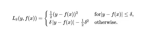
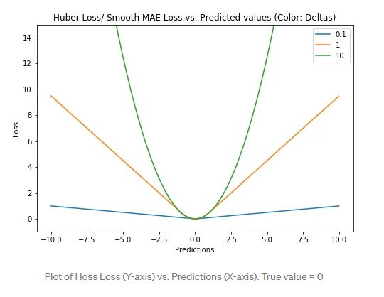
The choice of delta is critical because it determines what you’re willing to consider as an outlier. Residuals larger than delta are minimized with L1 (which is less sensitive to large outliers), while residuals smaller than delta are minimized “appropriately” with L2.
Why use Huber Loss
Using MAE for neural networks may lead to missing the minima when using gradient descent while MSE there is a gradient decrease as the loss gets close to its minima making it more precise. Huber loss curves around the minima which decreases the gradient.
It is more robust to outliers than MSE and therefore combines good properties from both MSE and MAE.
The only challenge is the need for tuning hyperparameter delta which is an iterative process.
Log-cosh is another function used in regression tasks that’s smoother than L2. Log-cosh is the logarithm of the hyperbolic cosine of the prediction error.
Advantage
log(cosh(x)) is approximately equal to (x ** 2) / 2 for small x and to abs(x) - log(2) for large x. This means that 'logcosh' works mostly like the mean squared error, but will not be so strongly affected by the occasional wildly incorrect prediction. It has all the advantages of Huber loss, and it’s twice differentiable everywhere, unlike Huber loss.
Many ML model implementations like XGBoost use Newton’s method to find the optimum, which is why the second derivative (Hessian) is needed. For ML frameworks like XGBoost, twice differentiable functions are more favorable.
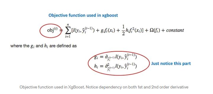
But Log-cosh loss isn’t perfect. It still suffers from the problem of gradient and hessian for very large off-target predictions being constant, therefore resulting in the absence of splits for XGBoost.
Quantile-based regression aims to estimate the conditional “quantile” of a response variable given certain values of predictor variables. Quantile loss is actually just an extension of MAE (when the quantile is 50th percentile, it is MAE).
Knowing about the range of predictions as opposed to only point estimates can significantly improve decision making processes for many business problems. Prediction interval from least square regression is based on an assumption that residuals (y — y_hat) have constant variance across values of independent variables. We can not trust linear regression models that violate this assumption.
We can not also just throw away the idea of fitting a linear regression model as the baseline by saying that such situations would always be better modeled using non-linear functions or tree-based models. This is where quantile loss and quantile regression come to the rescue as regression-based on quantile loss provides sensible prediction intervals even for residuals with non-constant variance or non-normal distribution.
The idea is to choose the quantile value based on whether we want to give more value to positive errors or negative errors. Loss function tries to give different penalties to overestimation and underestimation based on the value of the chosen quantile (γ). For example, a quantile loss function of γ = 0.25 gives more penalty to overestimation and tries to keep prediction values a little below median
Sources


